


In Machine Learning the best way to learn it is to write all common algorithms from scratch — without using any libraries like Scikit. Let’s write some most commonly used algorithms.
Let’s start with understanding the difference between Linear Regression and Logistic Regression and when to use them.
To put it in very simple words — when the prediction of outcome for the given input is in a range or continuous (i.e. regression), let’s say how many runs a batsman will hit in a match where the outcome in a continuous range, we can use Linear Regression.
While on the other hand, when the prediction of the outcome is in a discrete form (0 or 1) or the output is in the form of yes or no, logistic regression comes into play.
Like any machine learning model, we have three major topics on which the entire model stands.
1. Hypothesis
The hypothesis of logistic regression starts with linear regression where linear regression algorithm is used to predict y(range of outputs) for given x(inputs). However confining up to linear regression model doesn’t make sense for hθ (x) to take values larger than 1 or smaller than 0, since as per our requirement it has to be y ∈ {0, 1}. To fix this, we will be plugging all values for y in our Logistic function or “Sigmoid function”. Once passing all those values from linear regression to sigmoid function we will get the output in 1 or 0
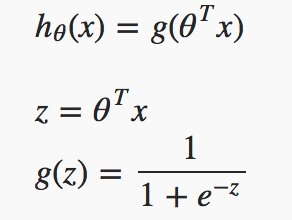
The hypothesis of logistic regression
If you can notice here, Z is nothing but matrix representation of the linear model, i.e. y = mx + c.
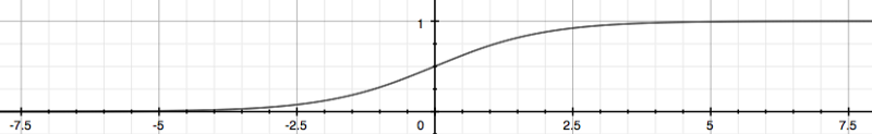
Sigmoid function
From the above graph, we can find that for any real number to the (0, 1) interval, making it useful for transforming an arbitrary-valued function into a function better suited for classification.
hθ (x) will give us the probability that our output is 1. For example,hθ (x)=0.7 gives us a probability of 70% that our output is 1. Our probability that our prediction is 0 is just the complement of our probability that it is 1 (e.g. if the probability that it is 1 is 70%, then the probability that it is 0 is 30%).
| z = np.dot(X, self.theta) | |
| h = self._sigmoid(z) |
2. Cost function or Loss function
We have some random parameters (represented by theta in our notation) to initialise our cost function. We want to fit the values of weights or parameters in such a way that our model works well that means decreasing the cost will increase the maximum likelihood assuming that samples are drawn from an identically independent distribution.
Our cost function somehow looks like :
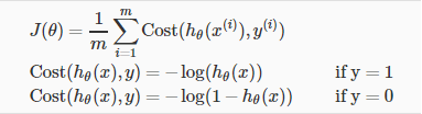
Logistic cost function
Another compact way to express above two conditions can be seen from the below code.
| def __loss(self, h, y): | |
| return (-y * np.log(h) – (1 – y) * np.log(1 – h)).mean() |
Let me help you in visualizing the cost function through a graph.
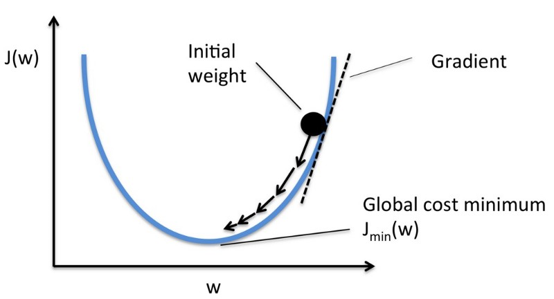
From the above graph, our goal is to reach the bottom-most point in the graph, and this can be achieved by adjusting our initial weight through gradient function and iterating the entire gradient function until the loss is minimized.
| gradient = np.dot(X.T, (h – y)) / y.size | |
| self.theta -= self.lr * gradient |
Minimizing gradient function
Now it’s time to predict our model, by calling our sigmoid function and getting probability > 0.5, we can consider such cases of class 1 and probability < 0.5 can be categorized as of class 0, so this is how the prediction of our model works.
| def _sigmoid(self,z): | |
| return 1 / (1 + np.exp(-z)) | |
| def predict(self, X,threshold=0.5): | |
| prob = self._sigmoid(np.dot(X, self.theta)) | |
| return prob >= self.threshold |
Sigmoid and predict function
This implementation is for binary logistic regression. For data with more than two classes, softmax regression has to be used. ( a blog post on that later)
Let me quickly summarise the entire story; we have started with the loading of data set in such a way that can be used for matrix calculation. We have designed our sigmoid function followed by our loss function.
Training our model with iterating linear model and plugging the output from linear function to our sigmoid function till we reach the minimum of cost or loss function. Once we train our model, we can work to predict and evaluate our model and hence we can calculate the loss and accuracy of our model.
Contact us today for more information
Anchit Jain -Technology Professional – Innovation Group – Big Data | AI | Cloud @YASH Technologies

Anchit Jain
Anchit Jain -Technology Professional – Innovation Group – Big Data | AI | Cloud @YASH Technologies
More From Author.


Related Posts.


AWS Cost Optimization Tips
Pravish Jain


Why one should adopt DataOps?
Pravish Jain

Multicloud strategy
Pravish Jain

Hybrid Environment – Gotchas
Pravish Jain


DevOps & DataOps best practices
Pravish Jain


Embrace the future of customer onboarding in banking
Sumeet Kulshreshth

Designing a seamless process for digitalizing customer onboarding in Banking
Sumeet Kulshreshth