

I have been exploring various machine learning algorithms like Linear Regression, Logistic Regression and Decision Trees for a while; it’s time for me to explore Neural Networks for advanced Machine Learning problems.
In this blog I’ll be discussing all the fundamentals of Machine learning(ML) and using this branch of science we will figure out how we can work on a problem where we need to predict something.
Let us start with understanding what Machine learning is?
Machine learning (ML) is a field of computer science that often uses statistical techniques to give computers the ability to “learn” (i.e., progressively improve performance on a specific task) with data, without being explicitly programmed.
Using the same concept we will try to train our model with a large dataset with all parameters, and at the end, we will test the model with some inputs.
A little theory for the big picture should not be painful.
We’ll try to precise every linked topic with minimal theory and maximum knowledge. Now how can we use ML (please excuse my laziness) for our problem statement and how we can use ML for this problem, and this is where the concept of Deep learning comes into play. In simple word deep learning is the way to implement ML using algorithms and inspired by the functionality of the brain called artificial neural networks.
Deep learning is an aspect of artificial intelligence (AI) that with emulating the learning approach that human beings use to gain acquire certain types of knowledge.
Did you see that? …. Artificial Neural Network. Yes please pay your attention here. It is a machine learning algorithm, which is built on the principle of the organization and functioning of biological neural networks. Now look at the beauty of ML here is that our entire neural network model will work in the same way like human brain work. Let us see what our dear google has to say about artificial neural networks.
An artificial neuron network (ANN) is a computational model based on the structure and functions of biological neural networks. Information that flows through the network affects the structure of the ANN because a neural network changes — or learns, in a sense — based on that input and output.
The below image briefs you about how a message is being transferred from one neuron to another where each neuron is located in a series of layer where we feed data to input layer and by passing it through successive hidden layer and training our model simultaneously we reach to layer called output layer where we can predict our output.
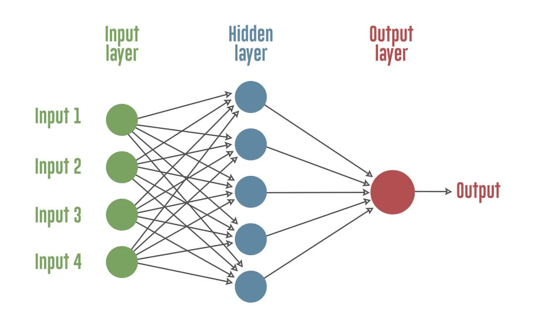
Artificial Neural Network
I guess this much theory suffices to learn our problem statement. It’s time to dive in our coding pool.
For those of you who want to understand Neural Networks in more depth — I’d recommend watching this short, yet exhaustive explanation of neural networks here.
Image classification:
The very first step in CNN is to classify the image since it very easy to visualise an image with human eye but how can we make the same thing to visualise through our machine …..Sad but machines can see :( this can be achieved through the matrix representation of the image. See how.
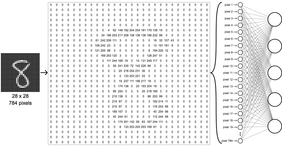
Image classification
From the above image, we can easily see the image (digit 8 ) now what is image nothing but the collection of pixels. So here the image consists 28 number of rows, and 28 number of columns which is equal to 784 pixels in total and these 784 pixels will act as an input to our first layer of CNN that is input layer. Similarly, we have taken thousands of images of dog and cat, and we have taken 150 by 150 pixels as input. Also, we rather than making each image one by one I have created a batch of images of size 16 for faster iteration. Taking samples of 2000 images in iterating the entire model for 50 (Epochs)
One Epoch is when an ENTIRE dataset is passed forward and backwards through the neural network only ONCE.
| from keras.preprocessing.image import ImageDataGenerator | |
| From keras.models import Sequential | |
| from keras.layers import Conv2D, MaxPooling2D | |
| from keras.layers import Activation, Dropout, Flatten, Dense | |
| from keras import backend as K | |
| # dimensions of our images. | |
| img_width, img_height = 150, 150 | |
| train_data_dir = ‘data/train’ | |
| validation_data_dir = ‘data/validation’ | |
| nb_train_samples = 2000 | |
| nb_validation_samples = 800 | |
| epochs = 50 | |
| batch_size = 16 | |
| if K.image_data_format() == ‘channels_first’: | |
| input_shape = (3, img_width, img_height) | |
| else: | |
| input_shape = (img_width, img_height, 3) |
Okay! Now we have designed our input layer and now moving ahead with further layers we choose our model to be sequential since the output of one layer is input to another layer and so on. Let’s check how these layers look like.
| model = Sequential() | |
| model.add(Conv2D(32, (3, 3), input_shape=input_shape)) | |
| model.add(Activation(‘relu’)) | |
| model.add(MaxPooling2D(pool_size=(2, 2))) | |
| model.add(Conv2D(32, (3, 3))) | |
| model.add(Activation(‘relu’)) | |
| model.add(MaxPooling2D(pool_size=(2, 2))) | |
| model.add(Conv2D(64, (3, 3))) | |
| model.add(Activation(‘relu’)) | |
| model.add(MaxPooling2D(pool_size=(2, 2))) | |
| model.add(Flatten()) | |
| model.add(Dense(64)) | |
| model.add(Activation(‘relu’)) | |
| model.add(Dropout(0.5)) | |
| model.add(Dense(1)) | |
| model.add(Activation(‘sigmoid’)) |
Let us see each function one by one….here we go.
- Sequential(): The sequential model is just a linear stack of layers. Add () method help you to add layers to your model.
- Conv2D : This layer creates a convolution kernel that is coiled with the input layer to produce a tensor (a generalization of matrices) of outputs.
- Activation: This function is a node between the output of one layer to another.
- MaxPooling2D : It is the process of down-sampling(reducing dimensions) the representation of the image.
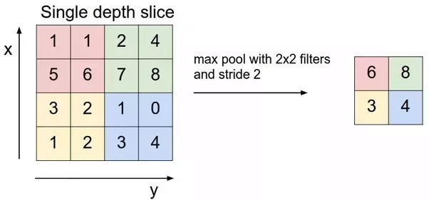
MaxPooling2D
Now once we have created the input and hidden layer, we need to connect all the layers to gain the output for that Flatten() method is used to take the input which creates 1-D array of input. Followed by Dense() method which is used to connect all the layers densely for the final output and the last method is Dropout() which is used to avoid overfitting.
Augmenting and Compiling the images :
This is something which helps in training our model with the best fit. Augmentation is the pre-processing of the image where a model is trained with a wide diversity of an image. This diversity of an image can be carried out in following ways like scaling, translation, rotation and flipping etc.
| # this is the augmentation configuration we will use for training | |
| train_datagen = ImageDataGenerator( | |
| rescale=1. / 255, | |
| shear_range=0.2, | |
| zoom_range=0.2, | |
| horizontal_flip=True) | |
| # this is the augmentation configuration we will use for testing: | |
| # only rescaling | |
| test_datagen = ImageDataGenerator(rescale=1. / 255) |
We then compile the CNN using the compile function. This function expects three parameters: the optimizer, the loss function, and the metrics of performance. The optimizer is the gradient descent algorithm we are going to use. We use the binary_crossentropy loss function since we are doing a binary classification.
Last, after gathering the well-structured data, it’s time to train the model. We have model.fit_generator() Where we take following arguments and train our model multiple times till we achieve the maximum accuracy and minimum loss. The accuracy of our model can be achieved by tuning our hyper-parameters (Epochs). Once we train our model with maximum accuracy, we need to save the whole model to avoid multiple training for every test.
| train_generator = train_datagen.flow_from_directory( | |
| train_data_dir, | |
| target_size=(img_width, img_height), | |
| batch_size=batch_size, | |
| class_mode=’binary’) | |
| print(train_generator.class_indices) | |
| validation_generator = test_datagen.flow_from_directory( | |
| validation_data_dir, | |
| target_size=(img_width, img_height), | |
| batch_size=batch_size, | |
| class_mode=’binary’) | |
| model.fit_generator( | |
| train_generator, | |
| steps_per_epoch=nb_train_samples // batch_size, | |
| epochs=epochs, | |
| validation_data=validation_generator, | |
| validation_steps=nb_validation_samples // batch_size) | |
| model.save(‘model.h5’) |
view raw train hosted with ❤ by GitHub
It’s time to summarize our learning’s so far and check out some necessary steps for building a dog-cat classifier.
- Image pre-processing
- Creating ANN layers
- Model training
- Model testing
- Model evaluation
Contact us today for more information
Anchit Jain -Technology Professional – Innovation Group – Big Data | AI | Cloud @YASH Technologies
Reference : en.wikipedia.org/wiki/Machine_Learning

Anchit Jain
Anchit Jain -Technology Professional – Innovation Group – Big Data | AI | Cloud @YASH Technologies
More From Author.

Related Posts.


AWS Cost Optimization Tips
Pravish Jain


Why one should adopt DataOps?
Pravish Jain

Multicloud strategy
Pravish Jain

Hybrid Environment – Gotchas
Pravish Jain


DevOps & DataOps best practices
Pravish Jain


Embrace the future of customer onboarding in banking
Sumeet Kulshreshth

Designing a seamless process for digitalizing customer onboarding in Banking
Sumeet Kulshreshth