SAP IBP’s Harmonized Planning Area: What It Means for Supply Chain Planning

Imagine running two parallel planning systems for the same supply chain — one for mid-to-long-term time series, another for short-term order-based execution, and synchronizing data between them and maintaining duplicate master data. Managing two sets of integrations. If you’ve ever implemented or operated SAP IBP, you know exactly the friction I’m describing.

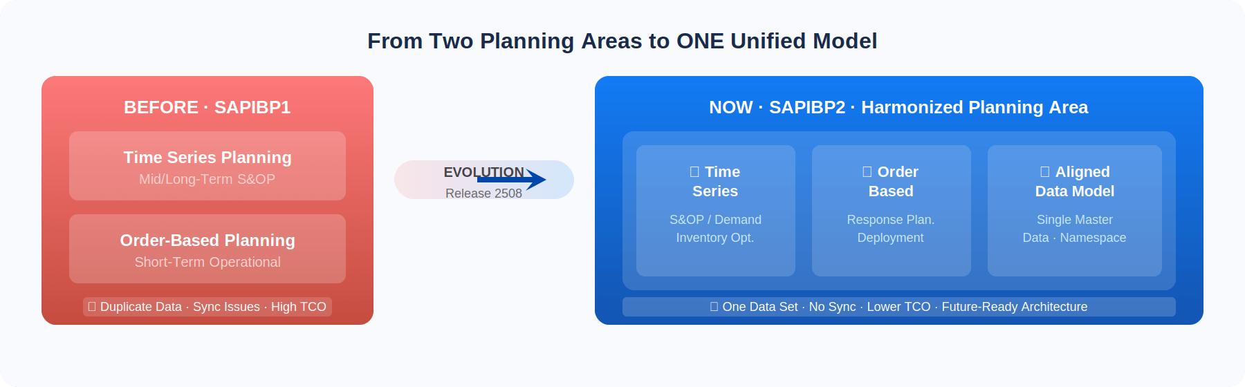
That ends with the Harmonized Planning Area (HPA) — SAP’s most architecturally significant step forward in IBP history, shipping in Release 2508. One planning area. One data model. One integration framework. And a future-proof backbone for everything that comes next.

Here’s a deep dive into what HPA actually is, how it works, and what it means for every supply chain professional working with SAP IBP today.

The Problem HPA Was Built to Solve

For years, SAP IBP customers running both time-series and order-based planning had to operate across two distinct planning areas:

• SAPIBP1 — the time-series home for S&OP, Demand Planning, and mid-term Inventory Optimization
• SAP7F (Order-Based) — the operational layer for Response Planning, Deployment, and Transportation Load Building

The cost of running both was enormous — not just in licensing or computing, but in:

• Duplicate master data loads (product, location, customer) that had to stay in sync
• Separate integration patterns for each planning area, each with its own error surface
• Data reconciliation overhead when time-series forecasts had to inform order-based execution
• UoM conversion inconsistencies between modules, causing accuracy drift in downstream plans
• Technical mismatches are preventing applications from sharing planning logic

“What is currently supported with two planning areas in customers’ implementation can now be done in one planning area — SAPIBP2 — with at least one proposed default integration technology.” — SAP IBP Product Documentation.

5 Innovations That Make HPA a Paradigm Shift

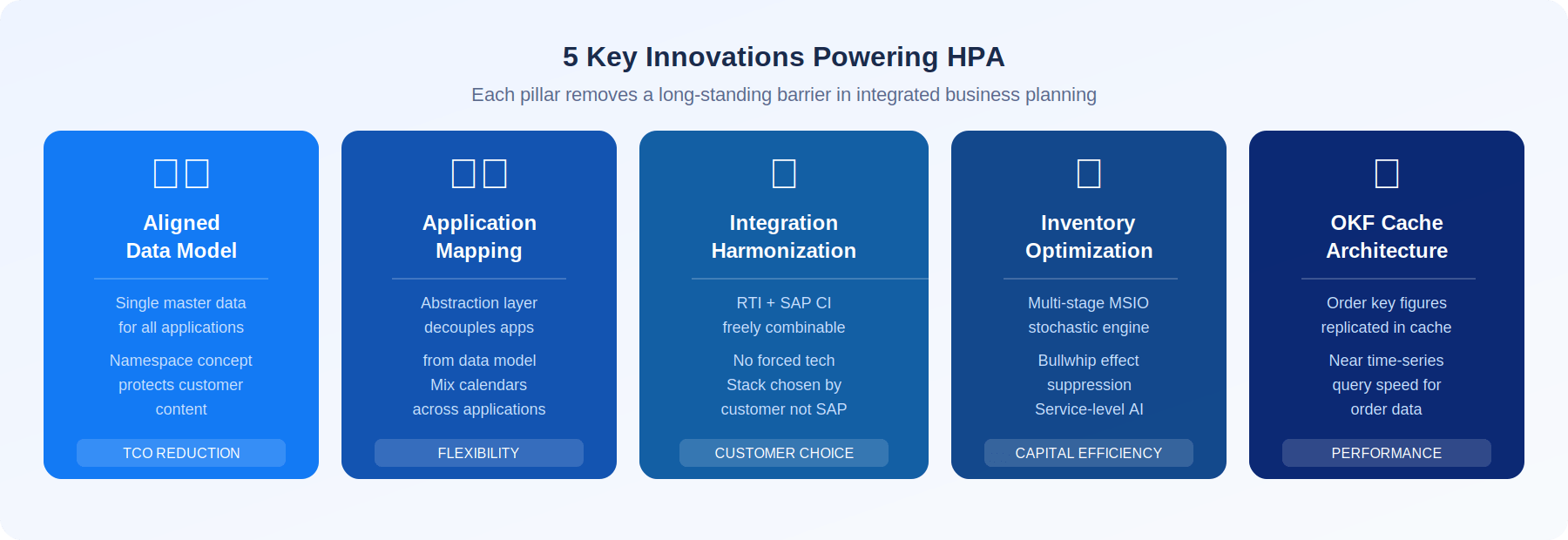
HPA is not a rebranding exercise. It involves a fundamental rearchitecting of five interconnected layers. Each layer removes a different category of structural limitation.

1 · The Aligned Data Model — The Heart of HPA

Every innovation in HPA flows from this: a single, unified data model that every application — Demand Planning, Inventory Optimization, Time-Series Supply, Order-Based Planning — understands and speaks natively.

SAP introduced a namespace concept to the SAPIBP2 planning area. Master data types, planning levels, attributes, and key figures all carry SAP’s namespace prefix (I_ for SAP-owned) rather than the customer namespace (without an underscore). This is not cosmetic — it prevents unintended overwrites of customer content by SAP or partner updates. Content protection is now structural.

The practical impact:

• One set of master data for all applications — no synchronization jobs between planning areas
• UoM conversions maintained once, centrally, via standard T006 table — eliminating the error-prone key figure conversion approach
• Future requirements can be shipped to the data model ahead of application consumption — meaning SAP can evolve the model incrementally without breaking existing implementations

Think of the aligned data model as moving from multiple city maps drawn by different cartographers to one canonical GPS that every navigation app uses.

2 · Application Mapping — Decoupling Apps from Data

The redesigned mapping layer is an abstraction layer that sits between the aligned data model and the application interfaces. Applications no longer reach directly into the planning area’s raw structure — they consume via a central mapping that the customer configures.

This unlocks real flexibility:

• A single Fiori app manages mapping for all applications — replacing multiple scattered mapping UIs
• Different applications can use different calendars in the same planning area (a previously painful constraint)
• The customer can remap SAP’s standard business meanings to custom attributes for application A while using different attributes for application
• Validation checks embedded in the mapping layer catch data type and length issues early — improving master data quality before it reaches planning
• Full visibility: a planner can see exactly which information each application consumes from a planning area with thousands of artifacts

3 · Integration Harmonization — Your Choice, Not SAP’s

This is the innovation that will reshape implementation projects. HPA offers a clean choice between two integration paths:

Real-Time Integration (RTI) uses bgRFC (background RFC) for transactionally consistent, sub-second synchronization of master and transactional data between S/4HANA and IBP. Any change to a Purchase Order, Sales Order, Stock Transfer Requisition, or Production Order in S/4HANA is captured, transformed, queued, and pushed to IBP automatically — no scheduled batch jobs. BAdI hooks provide transformation capability at the queue boundary in both directions.

SAP Cloud Integration (SAP CI) — part of the SAP Integration Suite on BTP — is the recommended path for new customers starting fresh with SAPIBP2. It is purely cloud-native, requires no agent, and supports end-to-end process integration through iFlows and API Management with separate subaccounts for dev, QA, and production.

The critical design decision in HPA is that the integration technology is now decoupled from the planning application. Previously, choosing Order-Based Planning effectively forced RTI. Now, a customer can run time-series supply planning with RTI master data feeds, or order-based planning via CI. The planning choice and the integration choice are orthogonal.

• For existing customers: CI-DS (Cloud Integration Data Services) remains supported
• For new customers starting SAPIBP2: SAP CI is the preferred path
• For customers with non-SAP or BW source systems: ETL integration remains available for master data and time-series historical data

4 · Inventory Optimization — Smarter Stock, Less Capital

SAP IBP’s Inventory Optimization within HPA is a self-developed, stochastic, non-linear optimization engine that simultaneously optimizes inventory across the entire end-to-end supply chain. The constraint: meet desired customer service levels. The objective is to minimize total inventory holding cost, treating internal service levels as decision variables—not fixed inputs.

What this means in practice:

• Bullwhip effect suppression: demand variability propagation to upstream stages is modeled explicitly, preventing the over-ordering cascades that plague multi-tier supply chains
• Internal service level optimization: the algorithm determines the optimal internal SL at each echelon, not the planner, resulting in significant inventory reductions
• Dynamic lead time integration: a dedicated supply lead time operator calculates transportation, production, and supplier lead time variability from historical data, feeding it as real input to the IO engine rather than using static estimates

In HPA, total average lead time and its variability are modeled as separate attributes at the header level — a cleaner model than SAPIBP1, where these were intermixed with operational activity modeling.

5 · Order Key Figure Cache (OKF Cache) — Performance at Scale

This is a technical innovation that planners will feel viscerally, even if they never know its name.

In current order-based planning, order key figures are calculated on the fly from OBP’s primary persistence, which accesses multiple master data tables and order tables per query. The calculation scenario procedures must be compiled each time—the result: slow Excel UI rendering, especially for key figures like Projected Stock.

The OKF Cache changes the access pattern. Order key figures are replicated into a cache structure that carries PERIODID and PLOBJID access — mimicking the single-table access pattern of time-series data. The query execution plan becomes lean. Compilation time drops. The Excel UI becomes significantly faster when working with order data.

This is achieved through dedicated job templates: Initial Loading of Order Key Figures (Cached), Reconcile Planning Objects, and consistency checks. The OKF cache must be initialized after migration and refreshed after significant data changes.

The Integration Architecture in Depth

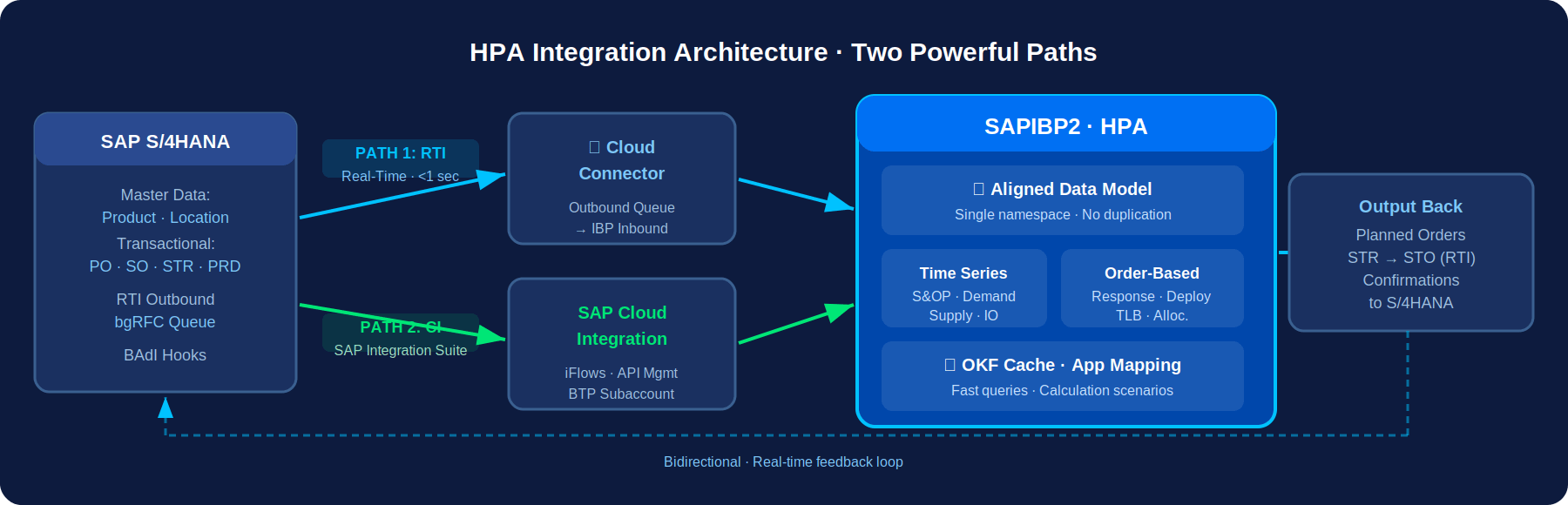
The RTI data flow is worth understanding in detail because it defines the real-time responsiveness envelope of your planning system:

1. Changes in S/4HANA (master or transactional data) are captured and stored in a bgRFC outbound queue
2. The Cloud Connector picks up the queue and sends it to IBP’s Inbound Queue in the cloud
3. IBP processes the inbound queue — data is persisted in application tables (master data, orders, stock)
4. Post-planning run, IBP supply elements (Planned Orders, STRs, etc.) are queued to RTI Outbound
5. Cloud Connector moves to S/4HANA Inbound Queue — BAdIs can transform on arrival
6. Supply elements are created in S/4HANA — STRs can be auto-converted to STOs for Deployment results

Important operational note: RTI is asynchronous. Queue errors block the data channel and prevent further transfer. Robust RTI monitoring — available in both IBP and ECC/S4 — is not optional in production. Build operations procedures for queue error resolution from Day 1.

The Key Figure Naming Convention — A New Language

HPA introduces a structured, transparent naming convention for key figures. Understanding it is essential for anyone doing functional configuration or custom development on SAPIBP2.

The fundamental distinction: stored key figures (time-series persistency) versus external/order key figures (order persistency) can never be stored in the same key figure object. They are separate persistencies. The naming scheme makes this explicit through suffixes:

• _OR suffix — order-based persistency (e.g., I_CAPACONSPLANNEDOR)
• _TS suffix — time-series persistency (e.g., I_CAPACONSPLANNEDTS)
• _LN or _PDS suffix — when a key figure exists at both lane and PDS granularity

The prefix structure encodes the business semantics:

• Constraint type/behavior: MIN, MAX, AVG, CALC, ADJ, FINAL
• Planning process: DISTR (distribution), PRODN (production), SUPPLY
• Status: PLANNED, FXD (fixed), UNFXD (unfixed), CONF (confirmed), CONFLATE
• Calculation detail: MEAN, CV, BIAS, COSTRT

This structure matters for architects and integration consultants: the naming convention tells you exactly which persistence layer a key figure sits in, which application it belongs to, and what its planning state is — just by reading the technical name.

Supply Planning in HPA — Heuristics, Optimization, and Order Fulfillment

Unconstrained Heuristics — Speed First

The infinite heuristic (unconstrained) is primarily a tool for data model validation and propagation. Since there are no capacity constraints, supply and demand are always aligned — making it the ideal first-pass operator to verify that your master data, sourcing rules, and transportation lanes are correctly configured before committing to a constrained run.

In HPA, heuristics use the Customer TLane Product master data to determine which DCs and plants can supply a given TSP customer. They calculate the dependent demand level by level, net demand at each node, and propagate to upstream production and procurement sources using T-Lane Product master data.

Supply Optimization — Cost-Based Planning at Scale

The optimizer transforms the supply planning problem into a Mixed Integer Linear Program (MILP). The solver finds the cost-optimal production, distribution, and procurement plan while respecting:

• Resource capacities (hard constraint)
• Sourcing options and availability (hard constraint)
• Safety stock targets (soft constraint — violation is costed)
• Quota arrangements (soft constraint — violation is costed)
• Min/max lot sizes (hard constraint)

Cost categories the optimizer weighs simultaneously:

• Demand side: Non-Delivery Cost, Late Delivery Cost (can be differentiated by customer segment)
• Supply side: Transportation Cost, Production Cost, Procurement Cost
• Inventory side: Safety Stock Violation Cost, Holding Cost
• Fixed costs: Prevent uneconomically small transport quantities

The optimizer uses abstract cost proportions, not currency values — the relationships between cost categories matter more than their absolute values. Getting the cost model right is the single most impactful implementation decision in supply optimization.

Order-Based Planning — The Operational Nerve Center

OBP in HPA runs four core processes, each executable independently or in combination, depending on business requirements:

• Supply & Allocation Creation: Generates allocations (demand caps per customer per period) and the baseline supply plan. Allocations enforce fair share in constrained scenarios.
• Response Planning: The short-term horizon engine — from the end of the frozen period to the response horizon end. Considers sales orders as hard demand, consumes allocations as constraints, creates order confirmations, and flags late/partial deliveries for RTI feedback to S/4HANA.
• Deployment Planning: Distributes confirmed available-to-deploy supply to demand elements using the Priority Deployment Heuristic. Creates Deployment STRs, which RTI converts to STOs for execution.
• Transportation Load Building (TLB): Groups planned distribution receipts into cost-optimized loads using equipment type constraints. Integrated with S/4HANA as multi-item requisitions via RTI outbound.

The Customer Model — Three Dimensions, One Planning Area

One of the most nuanced design decisions in HPA is the customer master data model. Because time-series and order-based planning serve different planning horizons with different granularity needs, HPA introduces three customer dimensions:

• TSP Customer (I_TSPCUSTID): The time-series planning dimension. A virtual grouping of business partners suitable for mid-to-long-term forecasting. Connected to locations via Transportation Lanes. Supports customer lead-time modeling and customer sourcing ratios.
• OBP Customer (I_OBPCUSTID): The operational dimension — the sold-to/ship-to business partner from ERP. Connected to a location through the forecast or sales order, not via a transportation lane. Reflects S/4HANA’s customer structure exactly.
• Customer Group (I_CUSTGROUP): The demand stream dimension for Inventory Optimization. Represents service-level management segments — e.g., strategic accounts, regional segments, channel tiers.

The implementation complexity of mapping TSP customers to OBP customers scales with supply chain size and structure:

• Low Complexity (small B2B, services): TSP and OBP customers map 1:1. No disaggregation needed. Direct attribute mapping. Virtualization is unnecessary.
• Medium Complexity (10k+ customers, equipment distribution): Customer groups are essential for S&OP discussion and IO SL management. Key accounts (Amazon, Walmart) forecasted individually; others grouped. Configuration: direct mapping plus disaggregation rules.
• High Complexity (CPG/Food, Life Sciences, 10k+ customers): Advanced segmentation by state/province or channel. Complex packaging/shelf life/regulatory dimensions. OBP expectation assessment is critical — what exactly is being integrated from IBP back to S/4HANA?

Unit of Measure Conversion — Finally Fixed

UoM conversion has been a persistent pain point in IBP implementations. Time-series planning and order-based planning handled conversions differently — time-series planning required all conversion factors to be uploaded to IBP; OBP relied on S/4HANA’s standard T006 table. The result was accuracy drift, configuration complexity, and unexpected reconciliation issues.

HPA introduces a central UoM conversion component accessible from both time-series and order-based applications. Key changes:

• Conversion factors are maintained once in the T006 standard table, reducing master data volume in IBP
• New attribute type “Unit of Measure” enables conversion object modeling in the planning area
• IBP_CONVERSION key figure calculation function simplifies conversion in custom key figure logic
• Every quantity continues to be stored in Base UoM throughout IBP — algorithms always receive unconverted data, eliminating the model error that occurred when the algorithm recalculated ETL-integrated order quantities
• Currency conversion is also centralized in the same Conversion Configurations section

The implications for existing customers: audit your current UoM conversion key figure calculations and CI-DS mapping before migrating to SAPIBP2. The new model is cleaner, but the migration requires deliberate data model mapping.

Release 2508 — What’s In, What’s Coming

Release 2508 is the foundation release for SAPIBP2, not the complete picture. SAP has been explicit about phased delivery:

Included in 2508

• Aligned data model with namespace concept
• Application mapping framework (central Fiori app)
• Inventory Optimization operators (most in scope for 2508)
• Time-series supply: heuristic and optimizer, recoded for new data model
• Order-based planning: full scope comparable to SAP7F (Response, Deployment, TLB, Allocation)
• RTI and SAP CI integration support
• OKF Cache architecture
• New production data model with a single I_PDSID key
• Single-tier vendor modeling (simplified)
• UoM conversion central component
• Customer product validity extension (T-Lane seasonality from release 2605)

Planned for Future Releases

• Multi-tier fully qualified vendor modeling (RTI-driven vendor product creation)
• Subcontracting in time-series supply planning
• Shelf life planning in OBP (shelf life removed from TS supply in SAPIBP2)
• Planned production resource substitution (alternate resources) in OBP
• Characteristic-based planning in OBP
• Source of supply validity (release 2605)
• Further heuristic/optimizer algorithm investments

What This Means for You — Practical Takeaways

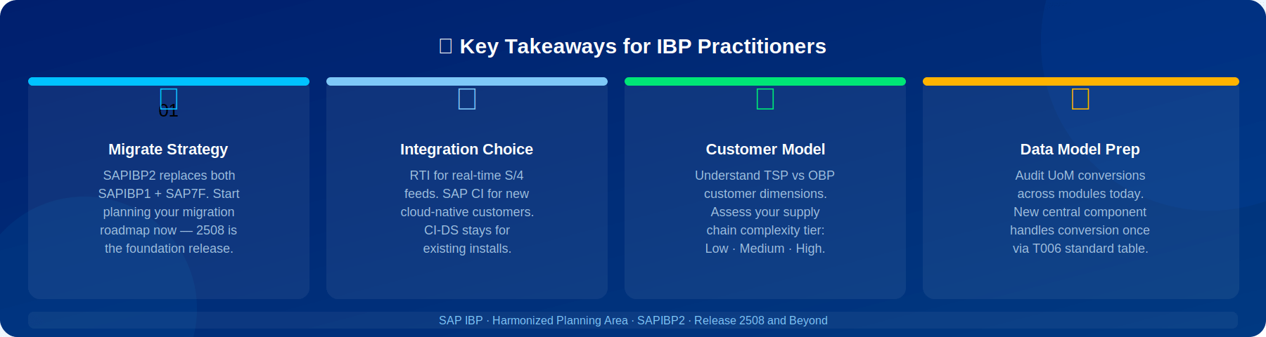
Whether you’re an IBP consultant, a supply chain architect, or a planning manager sponsoring an IBP program, here is where to focus your attention:

• If you are on SAPIBP1 only (time series): HPA gives you order-based capabilities you didn’t have. The question is when your roadmap justifies the move to SAPIBP2. Start by evaluating your short-term order fulfillment pain points — Response Planning may be the missing capability.
• If you are on SAP7F (order-based only): HPA unlocks S&OP-to-execution continuity. The 2508 release is the right time to plan the migration roadmap, especially if you’re on S/4HANA and can fully leverage RTI’s real-time capabilities.
• If you are running both SAPIBP1 + SAP7F: You’re the primary target for HPA. The business case is straightforward — fewer integrations, no data sync, a single master data source, and lower total cost. The migration complexity is real but manageable with phased planning.
• For new IBP implementations: Start on SAPIBP2. There is no reason to implement the old dual-area architecture when HPA is available. SAP CI is your integration path if you’re greenfield on S/4HANA.

The Bottom Line

The Harmonized Planning Area is not a release feature — it is a platform pivot. SAP has redesigned the foundational architecture of IBP to remove the structural limitations that have been holding back integrated planning for years.

The investment is substantial: a new data model, a new mapping framework, new engine APIs, new integration patterns, and a new performance architecture. None of this happens in a minor release. SAP is betting that this architecture will carry IBP forward for the next decade.

For supply chain professionals, the message is simple: understand this shift now so you can position your organization to benefit as the platform matures through 2508 and beyond.

🔵 If this resonated, drop a comment below — what’s your biggest pain point with the current dual planning area setup?

• SAPIBP
• SAPIntegratedBusinessPlanning
• SupplyChain